A Beginner’s Guide to Linear Regression in Machine Learning
2025-07-01 • 3 min read

Key Points
- Introduction
- What is Linear Regression?
- Example of Linear Regression
- Code Implementation
- Output of given example
- Conclusion
Introduction
When you think about predicting the future, whether it’s the price of a house, sales of a product, or the growth of a startup, Linear Regression is usually the first algorithm you’ll encounter.
It’s simple, powerful, and forms the foundation of many advanced machine learning techniques. In this blog, we’ll break down what linear regression is, how it works, and how to implement it with Python.
What is Linear Regression?
At its core, Linear Regression tries to draw the best straight line through a set of data points.
At its core, Linear Regression tries to draw the best straight line through a set of data points.
That line represents the relationship between:
Independent variable (X) → input (e.g., size of a house).
Dependent variable (Y) → output (e.g., price of a house).
The mathematical equation is:
Y = mX + b
Where:
- m = slope of the line (how much Y changes for each unit increase in X).
- b = intercept (the value of Y when X = 0).
Let's solve one example to understand clearly.
| X | Y |
|---|---|
| 1 | 50 |
| 2 | 55 |
| 3 | 65 |
| 4 | 70 |
| 5 | 75 |
Code: Implementation of Linear Regression
import numpy as np
import pandas as pd
import matplotlib.pyplot as plt
X = np.array([1, 2, 3, 4, 5])
Y = np.array([50, 55, 65, 70, 75])
# find summation of x
sumOfX = np.sum(X)
print("Summation of X: ",sumOfX)
# find summation of y
sumOfY = np.sum(Y)
print("Summation of Y: ",sumOfY)
# Product of x with y
prodOfXY = X * Y
print("Product of X with Y: ",prodOfXY)
# Summation of product of x with y
sumOfProdOfXY = np.sum(prodOfXY)
print("Summation of product of X with Y: ",sumOfProdOfXY)
# Square of X's value
squareOfX = X * X
print("Square of X: ",squareOfX)
# Summation of square of X
sumOfSquareOfX = np.sum(squareOfX)
print("Summation of square of X: ",sumOfSquareOfX)
# Find value of n
n = len(X)
print("Value of n: ",n)
# To calculate slope m
slope = slope = ((n * sumOfProdOfXY) - (sumOfX * sumOfY)) / ((n * sumOfSquareOfX) - ( sumOfX * sumOfX))
print("Slope: ",slope)
# To calculate b's value'
b = (sumOfY - (slope * sumOfX)) / n
print("b: ",b)
# I have every required value now so now predict Y
predY = slope * X + b
print("Predicted Y values:", predY)
# Enhanced DataFrame with more columns for analysis
df = pd.DataFrame({
'X': X,
'Original Y': Y,
'Predicted Y (Ŷ)': predY,
'Residual (Y - Ŷ)': Y - predY,
'X * Y': X * Y,
'X²': X ** 2
})
# Show the nicely formatted DataFrame
print("\nDetailed Linear Regression Table:\n")
print(df)
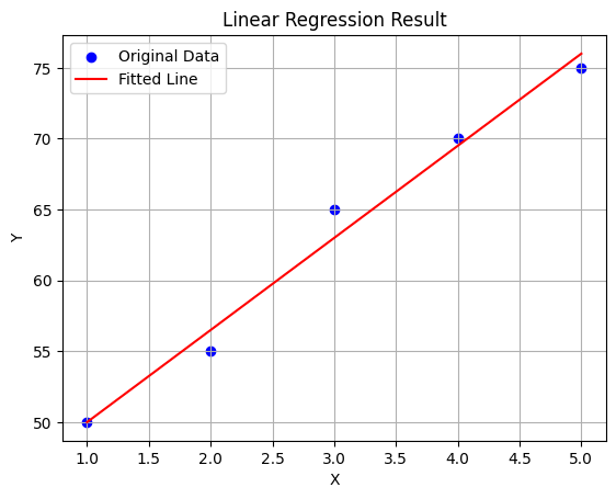
plt.scatter(X, Y, color='blue', label='Original Data')
plt.plot(X, predY, color='red', label='Fitted Line')
plt.xlabel('X')
plt.ylabel('Y')
plt.title('Linear Regression Result')
plt.legend()
plt.grid(True)
plt.show()
Output:
Summation of X: 15 Summation of Y: 315 Product of X with Y: [ 50 110 195 280 375] Summation of product of X with Y: 1010 Square of X: [ 1 4 9 16 25] Summation of square of X: 55 Value of n: 5 Slope: 6.5 b: 43.5 Predicted Y values: [50. 56.5 63. 69.5 76. ]
Detailed Linear Regression Table:
| X | Original Y | Predicted Y (Ŷ) | Residual (Y - Ŷ) | X * Y | X² |
|---|---|---|---|---|---|
| 1 | 50 | 50.0 | 0.0 | 50 | 1 |
| 2 | 55 | 56.5 | -1.5 | 110 | 4 |
| 3 | 65 | 63.0 | 2.0 | 195 | 9 |
| 4 | 70 | 69.5 | 0.5 | 280 | 16 |
| 5 | 75 | 76.0 | -1.0 | 375 | 25 |
Conclusion
Linear Regression is the "Hello World" of Machine Learning. It’s simple but incredibly powerful for understanding data patterns.